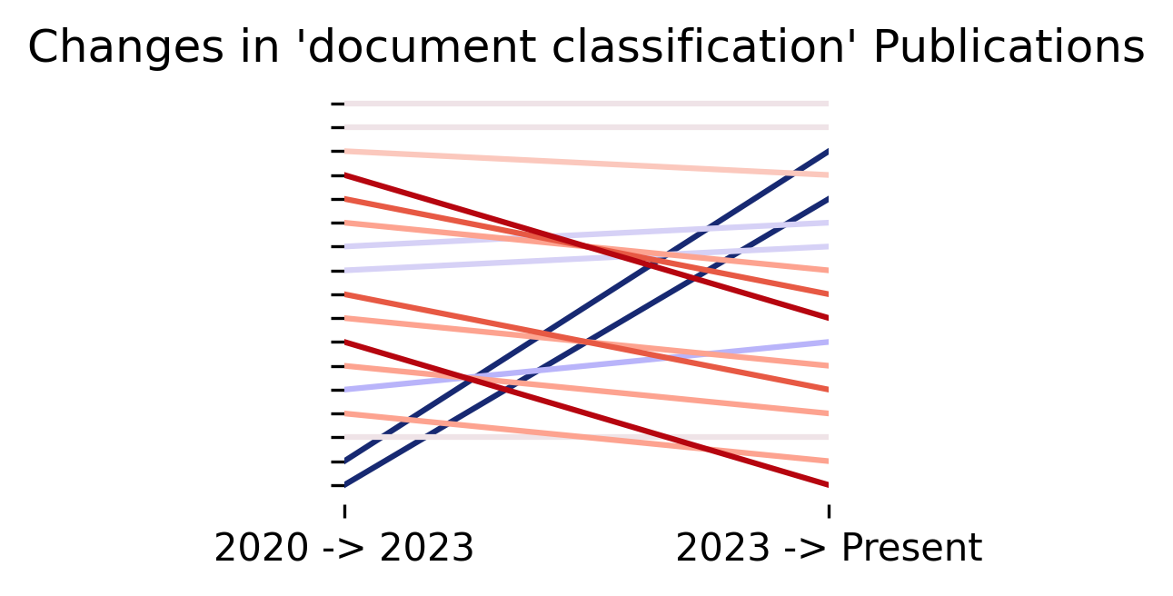
Changes in Novartis’ News Coverage
3 min
pip install sturdy-stats-sdk pandas numpy plotly duckdb colorcet
from IPython.display import display, Markdown, Latex
import pandas as pd
import numpy as np
import plotly.express as px
from sturdystats import Index, Job

from pprint import pprint## Basic Utilities
px.defaults.template = "simple_white" # Change the template
px.defaults.color_discrete_sequence = px.colors.qualitative.Dark24 # Change color sequence
def procFig(fig, **kwargs):
fig.update_layout(plot_bgcolor= "rgba(0, 0, 0, 0)", paper_bgcolor= "rgba(0, 0, 0, 0)",
margin=dict(l=0,r=0,b=0,t=30,pad=0),
**kwargs
)
fig.layout.xaxis.fixedrange = True
fig.layout.yaxis.fixedrange = True
return figindex = Index(id="112f567abe127f4502ec9ea0b9638faa")
# Uncomment the line below to create and train your own index
# index = Index(name="llms encode clinical knowledge cn")
if index.get_status()["state"] == "untrained":
index.ingestIntegration("cn_all", "https://www.nature.com/articles/s41586-023-06291-2")
index.train(dict(), fast=True)
print(job.get_status())
# job.wait() # Sleeps until job finishesFound an existing index with id="112f567abe127f4502ec9ea0b9638faa".Our bayesian probabilistic model learns a set of high level topics from your corpus. These topics are completely custom to your data, whether your dataset has hundreds of documents or billions. The model then maps this set of learned topics to single every word, sentence, paragraph, document, and group of documents to your dataset, providing a powerful semantic indexing.
This indexing enables us to store data in a granular, structured tabular format. This structured format enables rapid analysis to complex questions.
#index = Index(id="index_6095a26fc2be4674a005778dd8bcd5e5")
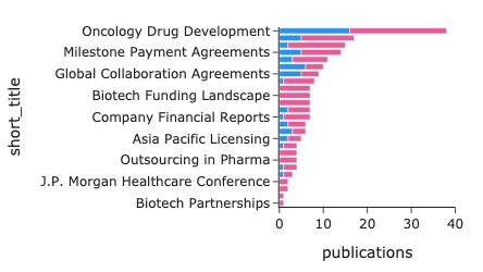
topic_df = index.topicSearch()
topic_df.head()| short_title | topic_id | mentions | prevalence | topic_group_id | topic_group_short_title | conc | entropy | |
|---|---|---|---|---|---|---|---|---|
| 0 | Link Prediction Algorithms | 42 | 327.0 | 0.081993 | 1 | Modeling and Prediction | 22.720280 | 5.585348 |
| 1 | Community Detection Methods | 24 | 279.0 | 0.074810 | 2 | Community and Social Networks | 25.426317 | 5.756143 |
| 2 | Stochastic Block Models | 12 | 184.0 | 0.046147 | 3 | Graph Theory and Analysis | 19.607786 | 6.206955 |
| 3 | Link Prediction Techniques | 64 | 240.0 | 0.043980 | 1 | Modeling and Prediction | 23.524736 | 4.783883 |
| 4 | Ecological Species Interactions | 88 | 66.0 | 0.036986 | 4 | Complex Systems and Applications | 19.529119 | 6.798615 |
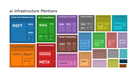
The following treemap visualizes the topics hierarchically: grouping the topics by the high level topic group. The size of each topic is porportional to the percentage of the time that topics shows up within papers about Transformer Architectures
fig = px.treemap(topic_df, path=["topic_group_short_title", "short_title"], values="prevalence", hover_data=["topic_id"])
procFig(fig, height=500).show()Let’s say we are interested in learning more about the years during which Radford Neal published papers on Adaptive Slice Samling. The topic information has been converted into a tabular format that we can directly query via sql. We expose the tables via the queryMeta api. If we choose to, we can do all of our semantic analysis directly in sql.
row = topic_df.loc[topic_df.short_title == "Ecological Species Interactions"]
row| short_title | topic_id | mentions | prevalence | topic_group_id | topic_group_short_title | conc | entropy | |
|---|---|---|---|---|---|---|---|---|
| 4 | Ecological Species Interactions | 88 | 66.0 | 0.036986 | 4 | Complex Systems and Applications | 19.529119 | 6.798615 |
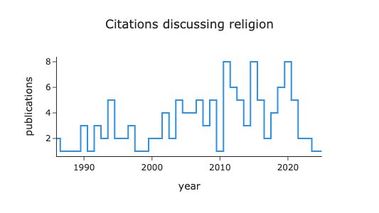
Because the semantic annotations are stored side by side with the metadata, we can further enrich our visualization and insights. We also have access to the citationCount of each publication.
df = index.queryMeta(f"""
SELECT
year(published::DATE) as year,
count(*) as publications,
median(citationCount) as median_citationCount
FROM doc
WHERE sparse_list_extract({row.iloc[0].topic_id+1}, sum_topic_counts_inds, sum_topic_counts_vals) > 2.0
GROUP BY year
ORDER BY year
""")
df["log Median Citation Count"] = np.log10(df.median_citationCount+1)
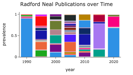
fig = px.bar(df, x="year", y="publications",
color="log Median Citation Count", color_continuous_scale="blues",
title=f"'{row.iloc[0].short_title}' Publications over Time", )
procFig(fig, title_x=.5)So far we have only looked at one topic at a time, However, we can perform much more complex analyses on our Our topics are stored in a tabular format alongside the metadata. This unified data storage enriches metadata with semantic information and enriches semantic information with structured context. As a result, we can perform complex semantic analysis with simple structured SQL queries
Below, we run a sql query to load the number of citations papers receive according to the sets of topics they belong to. The field theta is a sparse array broken up into theta_inds and theta_vals. theta_inds designates the list of topic_ids that appear in a document. theta_vals designates for each topic, what percentage of the document it comprises.
For each document, we unpack its topics. We then split its citations across topics porportional to the percentage of the document the topic comprises. We then do an agregration by topic id. This returns to us a list of topics and the median citation count associated with that topic
topicCitationsQuery = f"""
WITH t1 AS (
    SELECT
        unnest(theta_inds)-1 as topic_id, -- 1 indexed
        unnest(theta_vals) as topic_pct,
        citationCount,
        unnest(theta_vals)*citationCount as citationCount,
        year(published::DATE) as year
    FROM doc
)
SELECT
    topic_id,
    count(*) as publications,
    median(citationCount) as median_citationCount
FROM t1
WHERE topic_pct > .2
GROUP BY topic_id
ORDER BY median_citationCount desc
"""

topicCitations = index.queryMeta(topicCitationsQuery, paginate=True)
topicCitations.head(5)| topic_id | publications | median_citationCount | |
|---|---|---|---|
| 0 | 67 | 2 | 498.5 |
| 1 | 3 | 1 | 366.0 |
| 2 | 20 | 10 | 124.0 |
| 3 | 6 | 3 | 107.0 |
| 4 | 50 | 5 | 93.0 |
We can now return to our old Treemap visualization and imbue it with new information. Instead of assigning a color to each topic group, we can instead use a color scale to designate the median number of citations each topic received in our corpus. We convert the citation counts to log scale to support plotly’s built in linear continuous color scale.
The richer the blue, the more citations that topic tends to get. The richer the red, the fewer it tends to get.
import duckdb
import colorcet as cc


def buildDF(topicCitations):
    topic_df = index.topicSearch()
    df = duckdb.sql("""SELECT
        topic_df.*,
        topicCitations.publications,
        log(topicCitations.median_citationCount+1) as "log Median Citation Count"
    FROM topic_df
    INNER JOIN topicCitations
    ON topic_df.topic_id=topicCitations.topic_id
    """).to_df()

    ## For nicer color scale: most papers are between 10->1000
    df["log10 Median Citation Count"] = df["log Median Citation Count"].clip(1,2)
    return df

df = buildDF(topicCitations)
df["title"] = "Hierarchical Structure and the Prediction of Missing Links in Networks"
fig = px.treemap(df, path=["title", "topic_group_short_title", "short_title"],
                 values="publications",
                 color="log10 Median Citation Count", color_continuous_scale=cc.bgyw, )
fig = procFig(fig, height=500)
fig = fig.update_traces(hoverinfo='skip', hovertemplate=None)
figfrom sturdystats import Index
index = Index("Custom Analysis")
index.upload(df.to_dict("records"))
index.commit()
index.train()
# Ready to Explore
index.topicSearch()