Changes in Novartis’ News Coverage
3 min
pip install sturdy-stats-sdk pandas numpy plotly matplotlib
from IPython.display import display, Markdown, Latex
import pandas as pd
import numpy as np
import plotly.express as px
from sturdystats import Index, Job
import matplotlib.pyplot as plt


from pprint import pprint## Basic Utilities
px.defaults.template = "simple_white" # Change the template
px.defaults.color_discrete_sequence = px.colors.qualitative.Dark24 # Change color sequence
def procFig(fig, **kwargs):
fig.update_layout(plot_bgcolor= "rgba(0, 0, 0, 0)", paper_bgcolor= "rgba(0, 0, 0, 0)",
margin=dict(l=0,r=0,b=0,t=30,pad=0),
title_x=.5,
**kwargs
)
fig.layout.xaxis.fixedrange = True
fig.layout.yaxis.fixedrange = True
return fig
def displayText(df, highlight):
def processText(row):
t = "\n".join([ f'1. {r["short_title"]}: {int(r["prevalence"]*100)}%' for r in row["paragraph_topics"][:5] ])
x = row["text"]
res = []
for word in x.split(" "):
for term in highlight:
if term in word.lower() and "**" not in word:
word = "**"+word+"**"
res.append(word)
return f"<em>\n\n#### Result {row.name+1}/{df.index.max()+1}\n\n#### {row['title']} {row['published']}\n\n"+ t +"\n\n" + " ".join(res) + "</em>"
res = df.apply(processText, axis=1).tolist()
display(Markdown(f"\n\n...\n\n".join(res)))index = Index(id="index_b6a5a6ffb51e4ed695e80b92a8252a09")Found an existing index with id="index_b6a5a6ffb51e4ed695e80b92a8252a09".Our bayesian probabilistic model learns a set of high level topics from your corpus. These topics are completely custom to your data, whether your dataset has hundreds of documents or billions. The model then maps this set of learned topics to single every word, sentence, paragraph, document, and group of documents to your dataset, providing a powerful semantic indexing.
This indexing enables us to store data in a granular, structured tabular format. This structured format enables rapid analysis to complex questions. Our topic search api returns a ranked list of the most prominent topics in the corpus. The data includes a topic title, a group title, a topic_id, the discrete number of paragraphs that each topic was mentioned, and the percentage of data that is tied to each topic.
df = index.topicSearch()
df.head()[["short_title", "topic_group_short_title", "topic_id", "prevalence", "mentions"]]| short_title | topic_group_short_title | topic_id | prevalence | mentions | |
|---|---|---|---|---|---|
| 0 | Performance Enhancement Methods | Optimization Techniques | 186 | 0.046857 | 81545.0 |
| 1 | Innovations in Machine Learning | Machine Learning Techniques | 272 | 0.034884 | 50900.0 |
| 2 | Computational Efficiency Techniques | Optimization and Efficiency | 81 | 0.033749 | 61648.0 |
| 3 | Theoretical Foundations in Machine Learning | Theoretical Foundations | 325 | 0.032269 | 63637.0 |
| 4 | Performance Analysis | Evaluation and Assessment | 444 | 0.016385 | 31990.0 |
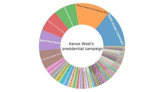
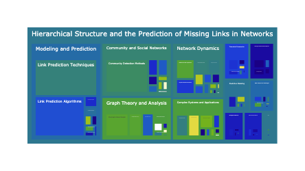
We can see there are two levels of topics: short_title and topic_group_short_title. The topic group is a high level thematic category while a topic is a much more granlular annotation. A dataset can have hundreds of topics, but ussually only 20-50 topic groups. This hierarchy is extremly useful for organizing and exploring data in hierarchical formats such as sunbursts.
The inner circle of the sunburst is the title of the plot. The middle layer is the topic groups. And the leaf nodes are the topics that belong to the corresponding topic group. The size of each node is porportional to how often it shows up in the dataset.
df["title"] = "ArXiv cs.LG Publications"
fig = px.sunburst(df, path=["title", "topic_group_short_title", "short_title"], values="prevalence", hover_data=["topic_id"],)
procFig(fig, height=550).show()Because we structure the semantic topics into a tabular format, we are able to store the data in a relational database. We expose this relational expose this structured sql functionality directly in our topicSearch api. In this case we can focus on ArXiv publications after 2022 to get a more modern view of ArXiv’s topics.
df = index.topicSearch(filters="published > '2022-01-01'")
df["title"] = "ArXiv cs.LG Publications <br> 2022-Present"
fig = px.sunburst(df, path=["title", "topic_group_short_title", "short_title"], values="prevalence", hover_data=["topic_id"],)
procFig(fig, height=550).show()We can actually see some meaningful changes between the first and second plot. Machine Learning Techniques overtook Optimization Techniques as the most prominent research publication topic. This is interesting. However, this is not most efficient way to visualize trends or changes over time.
Let’s do a comparison of trends within the most recent decade. We will be building constructing a slope plot made popular by data visualization pioneer Edware Tufte. This visualization enables us to view changes between two periods of time of extremely multidimensional data.
The first step is to collect a ranked list of topics for each time period. We simply need to do two topicSearch requests, one for each time period of interest. We now have a set of ranked topics for each time period
year1 = "2023"
year2 = "2020"

df1 = index.topicSearch(filters=f"published>'{year1}-01-01'", limit=512)
df2 = index.topicSearch(filters=f"published>'{year2}-01-01' and published<'{year1}-01-01'", limit=512)

df1.head()| short_title | topic_id | mentions | prevalence | one_sentence_summary | executive_paragraph_summary | topic_group_id | topic_group_short_title | conc | entropy | |
|---|---|---|---|---|---|---|---|---|---|---|
| 0 | Innovations in Machine Learning | 272 | 38618.0 | 0.062545 | Recent advancements in machine learning techni... | The recent surge in research reflects a concer... | 0 | Machine Learning Techniques | 7560.764160 | 6.038858 |
| 1 | Performance Enhancement Methods | 186 | 39289.0 | 0.050317 | Recent research focuses on innovative methods ... | The collected examples illustrate a strong emp... | 11 | Optimization Techniques | 9338.208984 | 5.675065 |
| 2 | Computational Efficiency Techniques | 81 | 27472.0 | 0.032877 | The examined documents focus on various method... | The recurring theme in the provided documents ... | 14 | Optimization and Efficiency | 1379.894897 | 5.978845 |
| 3 | Theoretical Foundations in Machine Learning | 325 | 26475.0 | 0.028910 | The recurring theme explores the intricate rel... | Throughout modern machine learning research, t... | 39 | Theoretical Foundations | 237.442551 | 6.499838 |
| 4 | Aligning Language Models | 223 | 9246.0 | 0.020157 | The theme revolves around enhancing the perfor... | The discussed theme centers on the continual d... | 54 | Natural Language Processing | 15.182971 | 5.556369 |
From there, we simply need to join the data so that for each topic, we know its current rank and previous rank. We also go ahead and annotate the two time periods for the data visualization
def joinDFs(df1, df2, N=40):
    ## Fiter the N most prominent topics in each period
    topic_ids = set(df1.head(N).topic_id.tolist() + df2.head(N).topic_id.tolist() )
    def procDF(df):
        df = df.loc[df.topic_id.apply(lambda x: x in topic_ids)].copy().reset_index(drop=True)
        df["Rank"] = df.index
        return df.sort_values("Rank")
    df1 = procDF(df1)
    df2 = procDF(df2)

    tid_to_info = df2.set_index("topic_id", drop=False).to_dict()
    df1["old_Rank"] = df1.topic_id.apply(lambda x: tid_to_info["Rank"][x])

    ## Annotate Time Periods
    df1["year"] = f"{year1} -> Present"
    df1["old_year"] = f"{year2} -> {year1}"
    df1["old_short_title"] = df2.short_title
    return df1[["topic_id", "old_Rank", "Rank", "short_title", "year", "old_year", "old_short_title"]]

joinDF = joinDFs(df1.copy(), df2.copy())
joinDF.head()| topic_id | old_Rank | Rank | short_title | year | old_year | old_short_title | |
|---|---|---|---|---|---|---|---|
| 0 | 272 | 12 | 0 | Innovations in Machine Learning | 2023 -> Present | 2020 -> 2023 | Performance Enhancement Methods |
| 1 | 186 | 0 | 1 | Performance Enhancement Methods | 2023 -> Present | 2020 -> 2023 | Computational Efficiency Techniques |
| 2 | 81 | 1 | 2 | Computational Efficiency Techniques | 2023 -> Present | 2020 -> 2023 | Theoretical Foundations in Machine Learning |
| 3 | 325 | 2 | 3 | Theoretical Foundations in Machine Learning | 2023 -> Present | 2020 -> 2023 | Performance Analysis |
| 4 | 223 | 47 | 4 | Aligning Language Models | 2023 -> Present | 2020 -> 2023 | Deep Learning Architectures |
From here we do a little processing to color our slopes: the darker the blue, the more the topic rose in prominence. The dark the red, the more it shrank in prominence. The more neutral colors stayed largely the same
from cmap import Colormap
cm = Colormap('colorcet:CET_D1A')

def prepareDF(df):
    ## Flip Rank
    df["Rank"] = df.Rank.max() - df.Rank
    df["old_Rank"] = df.old_Rank.max() - df.old_Rank
    ## Color according to change in Rank
    df["color"] = df.apply(lambda row: cm(
                1 - ( ((row["Rank"] - row["old_Rank"])/ (df.Rank.max())) + .5)
            ).hex,
     axis=1)
    return df

def buildPlot(df, title):
    # Create the plot
    fig, ax1 = plt.subplots(figsize=(4,10))
    for row in df.to_dict("records"):
        ax1.plot([row["old_year"], row["year"]], [row["old_Rank"], row["Rank"]], c=row["color"])
    ax1.set_yticks(df.index[::-1])
    ax1.set_yticklabels(df.old_short_title.to_list(), ha='right',)
    plt.tick_params(axis="y")
    ax1.set_xbound(0, 1)
    for spine in ax1.spines.values():
        spine.set_visible(False)
    ax1.set_title(title)
    return fig, ax1

fig, ax1 = buildPlot(prepareDF(joinDF), "Changes in cs.LG Publication Topics")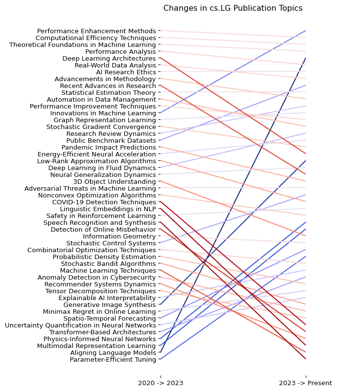
In addition to supporting arbitrary sql conditional logic, the topic search API also is also directly integrated to our probablistic search engine. The api accepts a search query parameter which performs a probablistic filter on each paragraph of the corpus before performing the topic rollup.
SEARCH_QUERY = "document classification"
year1 = "2023"
year2 = "2020"

df1 = index.topicSearch(SEARCH_QUERY, filters=f"published>'{year1}-01-01'", limit=512, semantic_search_cutoff=.6)
df2 = index.topicSearch(SEARCH_QUERY, filters=f"published>'{year2}-01-01' and published<'{year1}-01-01'", limit=512, semantic_search_cutoff=.6)

joinDF = joinDFs(df1.copy(), df2.copy(), 15)
fig, ax1 = buildPlot(prepareDF(joinDF.copy()), f"Changes in '{SEARCH_QUERY}' Publications")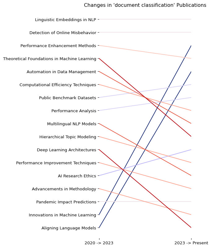
The topic search is an aggregration on top of our native search and tabular infrastructure and because topicSearch follows the same api parameters, we easily switch from an aggregate overview to specific examples
Let’s say we want to dig more into the Multimodal Representation Learning topic. We can easily surface all the matching examples from that went into the topic search results and line graph
row = df1.loc[df1.short_title == "Multimodal Representation Learning"]
row| short_title | topic_id | mentions | prevalence | one_sentence_summary | executive_paragraph_summary | topic_group_id | topic_group_short_title | conc | entropy | |
|---|---|---|---|---|---|---|---|---|---|---|
| 19 | Multimodal Representation Learning | 339 | 47.0 | 0.009339 | This theme explores the alignment and interact... | The provided documents illustrate the advancem... | 34 | Multimodal and Interactive Systems | 14.713141 | 5.465266 |
docdf = index.query(SEARCH_QUERY, topic_id=row.topic_id, filters=f"published>'{year1}-01-01'", semantic_search_cutoff=.6, limit=200)

## NB length of docs returned line up with number of mentions
assert len(docdf) == row.mentions.iloc[0]displayText(docdf.iloc[[0,-1]], [*SEARCH_QUERY.split(), "multi", "modal", "metadata", "graph", "layout""imgbert", "images"])
Document layout analysis (DLA) is the task of detecting the distinct, semantic content within a document and correctly classifying these items into an appropriate category (e.g., text, title, figure). DLA pipelines enable users to convert documents into structured machine-readable formats that can then be used for many useful downstream tasks. Most existing state-of-the-art (SOTA) DLA models represent documents as images, discarding the rich metadata available in electronically generated PDFs. Directly leveraging this metadata, we represent each PDF page as a structured graph and frame the DLA problem as a graph segmentation and classification problem. We introduce the Graph-based Layout Analysis Model (GLAM), a lightweight graph neural network competitive with SOTA models on two challenging DLA datasets - while being an order of magnitude smaller than existing models. In particular, the 4-million parameter GLAM model outperforms the leading 140M+ parameter computer vision-based model on 5 of the 11 classes on the DocLayNet dataset. A simple ensemble of these two models achieves a new state-of-the-art on DocLayNet, increasing mAP from 76.8 to 80.8. Overall, GLAM is over 5 times more efficient than SOTA models, making GLAM a favorable engineering choice for DLA tasks.
…
Memes are a popular form of communicating trends and ideas in social media and on the internet in general, combining the modalities of images and text. They can express humor and sarcasm but can also have offensive content. Analyzing and classifying memes automatically is challenging since their interpretation relies on the understanding of visual elements, language, and background knowledge. Thus, it is important to meaningfully represent these sources and the interaction between them in order to classify a meme as a whole. In this work, we propose to use scene graphs, that express images in terms of objects and their visual relations, and knowledge graphs as structured representations for meme classification with a Transformer-based architecture. We compare our approach with ImgBERT, a multimodal model that uses only learned (instead of structured) representations of the meme, and observe consistent improvements. We further provide a dataset with human graph annotations that we compare to automatically generated graphs and entity linking. Analysis shows that automatic methods link more entities than human annotators and that automatically generated graphs are better suited for hatefulness classification in memes.
from sturdystats import Index

index = Index("Custom Analysis")
index.upload(df.to_dict("records"))
index.commit()
index.train()

# Ready to Explore
index.topicSearch()