Transformer Architecture Structured Citations
3 min
pip install sturdy-stats-sdk pandas numpy plotly
from IPython.display import display, Markdown, Latex
import pandas as pd
import numpy as np
import plotly.express as px
from sturdystats import Index, Job

from pprint import pprint

index_id = "index_6a3d7feae6f142f496524be74010e9ee" ## Optionally Replace with your own Earnings Call Index
index = Index(id=index_id) # Visit sturdystatistics.com to get your free API key
Found an existing index with id="index_6a3d7feae6f142f496524be74010e9ee".## Basic Utilities
px.defaults.template = "simple_white" # Change the template
px.defaults.color_discrete_sequence = px.colors.qualitative.Dark24 # Change color sequence
def procFig(fig, **kwargs):
fig.update_layout(plot_bgcolor= "rgba(0, 0, 0, 0)", paper_bgcolor= "rgba(0, 0, 0, 0)",
margin=dict(l=0,r=0,b=0,t=30,pad=0),
**kwargs
)
fig.layout.xaxis.fixedrange = True
fig.layout.yaxis.fixedrange = True
return fig
def displayText(df, highlight):
def processText(row):
t = "\n".join([ f'1. {r["short_title"]}: {int(r["prevalence"]*100)}%' for r in row["paragraph_topics"][:5] ])
x = row["text"]
res = []
for word in x.split(" "):
for term in highlight:
if term in word.lower() and "**" not in word:
word = "**"+word+"**"
res.append(word)
return f"<em>\n\n#### Result {row.name+1}/{df.index.max()+1}\n\n#### {row['title']} {row['published']}\n\n"+ t +"\n\n" + " ".join(res) + "</em>"
res = df.apply(processText, axis=1).tolist()
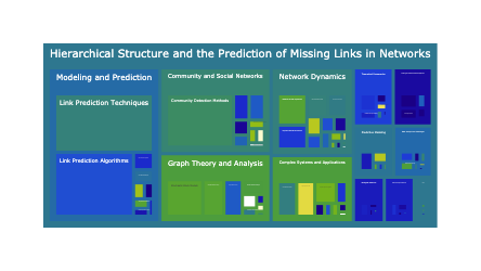
display(Markdown(f"\n\n...\n\n".join(res)))Our bayesian probabilistic model learns a set of high level topics from your corpus. These topics are completely custom to your data, whether your dataset has hundreds of documents or billions. The model then maps this set of learned topics to single every word, sentence, paragraph, document, and group of documents to your dataset, providing a powerful semantic indexing.
This indexing enables us to store data in a granular, structured tabular format. This structured format enables rapid analysis to complex questions.
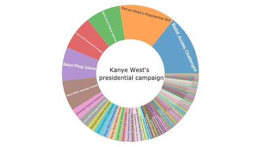
The inner circle of the sunburst is the title of the plot. The middle layer is the topic groups. And the leaf nodes are the topics that belong to the corresponding topic group. The size of each node is porportional to how often it shows up in the dataset.
SEARCH_QUERY = "novartis"
df = index.topicSearch(SEARCH_QUERY, semantic_search_cutoff=.3)
df["title"] = f"{SEARCH_QUERY} News"
fig = px.sunburst(df, path=["title", "topic_group_short_title", "short_title"], values="prevalence", hover_data=["topic_id"])
procFig(fig, height=500).show()We can select any point above and pull out the actual excerpts that comprise it. Let’s say we are interested diving into the topic Advancements in Treatment Options (topic 282). We can easily query our index to pull out the matching excerpts.
This query is filtering on documents that match on novartis as well as the topic Advancements in Treatment Options (topic 282).
topic_id = 282
row = df.loc[df.topic_id==topic_id]
row| short_title | topic_id | mentions | prevalence | one_sentence_summary | executive_paragraph_summary | topic_group_id | topic_group_short_title | conc | entropy | title | |
|---|---|---|---|---|---|---|---|---|---|---|---|
| 9 | Advancements in Treatment Options | 282 | 51.0 | 0.021055 | The recent FDA approvals highlight significant... | Recent press releases from pharmaceutical comp... | 0 | Pharmaceutical Innovations | 3354.828613 | 5.584366 | novartis News |
docdf = index.query(SEARCH_QUERY, topic_id=topic_id, semantic_search_cutoff=.3, limit=100, max_excerpts_per_doc=100)
print("Search:", SEARCH_QUERY, "Topic:", row.short_title.iloc[0])
displayText(docdf.iloc[[0, -1]], highlight=[*SEARCH_QUERY.split(), "generative", "model", "data", "center",])

## NB the number of excerpts lines up with the number of mentions
assert len(docdf) == row.mentions.iloc[0]
Search: novartis Topic: Advancements in Treatment Options
Having overcome what the global oncology and hematology chief calls “manufacturing hiccups” after the approval of Pluvicto in 2022, Legos is confident the companies that are just now discovering the modality will have a tough time building the scale that Novartis has. The pharma also has Lutathera on the market for certain gastroenteropancreatic neuroendocrine tumors.
…
Novartis president for US Victor Bultó said: “The U.S. approval of Fabhalta is an extraordinary moment for people living with PNH, their loved ones and the healthcare providers who care for them.
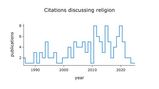
Sturdy Statistics integrates its semantic search directly into its sql api, enabling powerful sql analyses. Let’s quickly explore how many news articles were discussing novertis over the past year.
SEARCH_QUERY = "novartis"
df = index.queryMeta("SELECT date_trunc('month', TRY_CAST(published AS DATE)) as month, count(*) as mentions \
FROM paragraph WHERE published > '2024-01-01' GROUP BY month ORDER BY month ",
                     search_query=SEARCH_QUERY, semantic_search_cutoff=.1)
fig = px.bar(df, x="month", y="mentions",title=f"Mentions of '{SEARCH_QUERY}'")
procFig(fig, title_x=.5).show()Let’s saw we want to dive into novartis’s news coverage and discover the topics whose coverage has increased a meaningful amount over the past few months. We could turn to the topicSearch api, pass in two different filters and do a statistical test on every topic. Or we could use the topicDiff api.
The topic diff api extracts topics in some defined GROUP1 that has increased relative to some other GROUP2. Each group is defined by a sql conditional filter and a search query. The api then returns a list of topics in a similar style to topicSearch ordered by the confidence that the topic has increased in group 1 relative to group2. This api enables extremely powerful, denoised semantic comparisons on arbitrary sets of filters.
Below, we define filter1 as all documents published between Nov 2024 and Feb 2025, and we define filter2 as all documents published between Sept 2024 and Nov 2024. Additionally, we filter both groups by the search_query novartis because we want our comparison to be entirely limitted to articles that discuss novartis.
filter1 = "published > '2024-11-01'  AND published < '2025-02-01'",
filter2 = "published < '2024-11-01'  AND published > '2024-09-01'",

df = index.topicDiff(
    filter1=filter1,
    filter2=filter2,
    search_query1="novartis",
    search_query2="novartis",
    semantic_search_cutoff=.2,
    semantic_search_weight=.5
)
df1 = df[["short_title", "mentions", "comparative_mentions"]].copy()
df2 = df1.copy()
df1.head()| short_title | mentions | comparative_mentions | |
|---|---|---|---|
| 0 | Oncology Drug Development | 38.0 | 16.0 |
| 1 | Milestone Payment Agreements | 14.0 | 5.0 |
| 2 | Pharma Mergers & Acquisitions | 17.0 | 5.0 |
| 3 | Gene Therapy for Duchenne Muscular Dystrophy | 15.0 | 2.0 |
| 4 | Venture Capital Fundraising | 10.0 | 6.0 |
Below we can visualize the increase in mentions between group1 and group2. The mentions refers to the number of mentions of group1 (your group of interest) and comparative_mentions refers to the number of mentions of the topic within group two.
In the bar plot below, we plot the comparative mentions, along with the increase (delta) in mentions of that topic in our group1 filter.
df1["publications"] = df1.mentions - df2.comparative_mentions
df2["publications"] = df2.comparative_mentions
df1["label"] = "Delta"
df2["label"] = "Baseline"
resdf = pd.concat([df1, df2]).sort_values(["mentions", "label"], ascending=True)

fig = px.bar(resdf, y="short_title", x="publications", color="label")
fig = procFig(fig, height=500)
figfrom sturdystats import Index
index = Index("Custom Analysis")
index.upload(df.to_dict("records"))
index.commit()
index.train()
# Ready to Explore
index.topicSearch()